Methodology
Data Preparation
The Taricha granulosa sample data downloaded from BISON contained more than 12400 recorded newt sightings in the Pacific Northwest as a CSV file. To prepare the data for Maxent, all columns were deleted except for species name, x-coordinate, and y-coordinate. Data that was removed from the file included information such as time and date, identify of observer, organization of observer, state/province, county, and city. The next step was to filter out all entries that were missing coordinate data. Using an Excel function, the list was narrowed down to 11394 entries. The species name column was then standardized as Taricha granulosa and saved as a comma separated values (.csv) file.
Current Distribution
As all spatial data and environmental variables downloaded were in GeoTiff format, they needed to be converted to ASCII text raster for Maxent. This was done in QGIS 3.12.1 Bucuresti using the Translate Raster function. Spatial resolution was maintained at 30 arc seconds.
Taricha granulosa data was added to Maxent as the sample data, while all eight converted environmental variables files were used as environmental data. The output was set as an ASCII file with a cloglog distribution. After running the model, it was discovered that with so many sample points clustered in a relatively small area, the sample point marks completely blocked out large portions of the output map. To rectify this, the model was run again with sample radius changed from 0 to -9, which resulted in the points disappearing. Resolution and datum were preserved at 30 arc seconds WGS 84.
Future Distribution Prediction
The jackknife test on the current distribution model showed that 97.4% of informational importance came from annual mean temperature, minimum temperature, and maximum precipitation, with all other variables accounting for less than 1% each. As such, the predictive models were run with only the three key variables for efficiency.
The environmental data used for the predictive models were climate schemes from the Geophysical Fluid Dynamics Laboratory’s Coupled Physical Model 3. CM3 models the atmosphere’s climate from 70m above the Earth’s surface to 80km at the top end (GFDL, n.d.). Exact temperature change patterns over time can be seen in the graph below (Fig. 1).
Fig. 1 Geophysical Fluid Dynamics Laboratory Coupled Physical Model 3 Climate Model Pathways
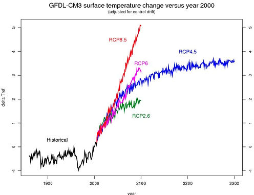
For future predictions, we used RCP (Representative Concentration Pathways) 4.5 and 8.5. These are IPCC approved climate projection models that model different potential climate change scenarios over the next century. RCP 4.5 models a greenhouse gas emissions peak at around 2040 before declining gradually. RCP 8.5 presents a worst-case scenario where emissions slow in growth over time slightly with technology but never fully halt. These two pathways were chosen as 4.5 is a highly likely scenario, being in the middle, while 8.5 presents the worst possible climate change landscape. 4 models were created in total: RCP 4.5 and 8.5 in 2050, and RCP 4.5 and 8.5 in 2070.
After running the maxent models, the output ASCII rasters were imported into ArcMap 10.6. The ArcMap data frame workspace was set as UTM Zone 10N Transverse Mercator projection. When the rasters were added, the coordinate system was set as WGS 1984 using the Define Projection tool, which was then projected on the fly to UTM Zone 10N. Canada and USA base maps from GADM were loaded and set to transparent to provide border lines. Maps were then created using ArcMap’s layout mode.
When analyzing the Maxent results in conjunction with land usage, we used Quick Stats from ENVI 5.3 to check the score distribution of all of our RCP 4.5 and RCP 8.5 outputs within our study area (BC, WA and OR). ENVI’s Quick Stats tell us the total number of pixels, the pixel’s DN value with its correspondent count, and its percentage of the entire raster data. In this case, we choose the pixels that have DN values that are greater than 0.7 as areas with good prediction accuracy. A value of 0.7 was selected as it is above 0.5, which is often regarded as the minimum threshold to constitute a habitat in species distribution modelling (Duan et al., 2014). Since the Maxent models are a cloglog distribution, a value of 0.7 lies at the upper end of the curve where change is greatest. Furthermore, 0.7 is also the value used by Kalboussi and Achour in their model of snake distribution (2018).
To exclude lands with high human activities or terrain unsuitable for newts, we used land cover data from the USGS’s Gap Analysis Project. The data was provided as a 30 m by 30 m raster. For the habitat niche maps, we use Raster Calculator from ArcGIS Pro 2.5 to limit the habitat niches to only those that scored higher than 0.7 for all of our 2000, 2050, and 2070 RCP 4.5 results. To identify the land cover types, we use ArcGIS Pro to create the attribute table for the land cover raster and join the table with the corresponding land use classifications. The extract by attribute tool from ArcGIS was used to keep the preferred land cover types. In this case, we kept the “Temperate Flooded & Swamp Forest”, “Tropical Flooded & Swamp Forest”, “Warm Temperate Forest & Woodland”, “Cool Temperate Forest & Woodland” and “Temperate to Polar Freshwater Marsh, Wet Meadow & Shrubland'' classes based on ideal newt habitats; places such as urban, shrub, crop fields, and alpine were all excluded from the land cover data. The last step was to use the Raster Calculator to identify the overlapping raster pixels of Maxent results and preferred land cover types. Maps from the three time periods were created using ArcGIS Pro's layout mode.